R plotting function for IRT model ICCs with user-specified parameter values

For teaching IRT, I created an R function for easy plotting of ICCs with user-specified parameter values. The function is called plot.ICCs, and it plots item characteristic curves for the Rasch, 2PL, 3PL and GRM model. The D value is 1.7 by default.

plot.ICCs <- function(a = NULL, b, c = 0, D = 1.7, single.item = TRUE) {
  k <- length(b)
  if(is.null(a)) {
    a <- rep(1, times = k) 
  }
  if(length(a) < k) {
    a <- rep(a, times = k)
  }
  if(length(c) < k) {
    c <- rep(c, times = k)
  }
  if(single.item == TRUE) {
    probs <- list()
    if (k == 1) {
      probs[[1]] <- function(theta, D = D, a, b1, c = 0) {
        c + (1-c) * (1 - (exp(-D * a * (theta - b1)) / (1 + exp(-D * a * (theta - b1)))))
      }
    }
    if(k > 1) { 
      probs[[1]] <- function(theta, D = D, a, b1, c = 0) {
        exp(-D * a * (theta - b1)) / (1 + exp(-D * a * (theta - b1)))
      }
      for (i in 2:(k-1)) {
        probs[[i]] <- function(theta, D = D, a, b1, b2, c = 0) {
          (exp(D * a * (theta - b1)) / (1 + exp(D * a * (theta - b1)))) -
            (exp(D * a * (theta - b2)) / (1+exp(D * a * (theta - b2))))
        }
      }
      probs[[k]] <- function(theta, D = D, a, b1, b2, c = 0) {
        (exp(D * a * (theta - b1)) / (1 + exp(D * a * (theta - b1))))
      }
    }
  }
  if(single.item == FALSE) {
    probs <- list()
    for (i in 1:k) {
      probs[[i]] <- function(theta, D = D, a, b, c) {
        c + (1 - c) * (1 / (1 + exp(-D * a * (theta - b))))
      }
    }
  }
  color <- c("black", "green", "red", "lightblue", "yellow", "purple", "pink", "brown")
  curve(probs[[1]](x, a = a[1], b = b[1], c = c[1], D = D), -4, 4, col = color[1], xlab = expression(theta), 
        ylab = "probability", ylim = c(0,1))
  if(k > 1) {
    if (single.item == TRUE)  {
      b <- c(b, Inf)   
      for (i in 2:k) {
        curve(probs[[i]](x, a = a[i], b1 = b[i], b2 = b[i+1], D = D), -4, 4, col = color[i], add = TRUE)
      }
    }
    if(single.item == FALSE) {
      for (i in 2:k) {
        curve(probs[[i]](x, a = a[i], b = b[i], c = c[i], D = D), -4, 4, col = color[i], add = TRUE)
      }
    }
  }
}

Here are some examples on how to use the function (images of some of the resulting plots are given below):

## 1PL model in logistic metric (default) for a single item:
plot.ICCs(b =.5) 
## 1PL model in normal metric for a single item:
plot.ICCs(b =.5, D = 1)  
## 2PL model for a single item:
plot.ICCs(b = .5, a = 1.5) 
## 3PL model for a single item:
plot.ICCs(b = .5, a = 1.5, c = 1/3)
## 3PL curves for three items:
plot.ICCs(b = c(-1, 0, .5), a = 1.5, c = 1/4, single.item = F) 
## 3PL curves for three items with different a and c parameters:
plot.ICCs(b = c(-1, 0, .5), a = c(.5, 1, 1.5), c = c(1/3, 1/2, 1/4), single.item = F) 
## a GRM model for 8 response categories (i.e., 7 thresholds):
plot.ICCs(a = 1, b = -3:3) 

## 1PL model in logistic metric for a single item:

## 3PL curves for three items with different a and c parameters:

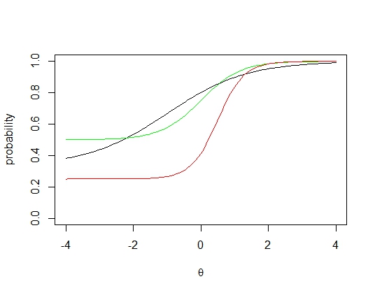
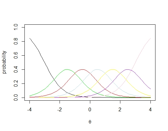
## a GRM model for 8 response categories (i.e., 7 thresholds):

This post was created with the help of: http://www.umass.edu/remp/software/simcata/wingen/modelsF.html for the probability ditribution functions http://www.craftyfella.com/2010/01/syntax-highlighting-with-blogger-engine.html for showing how to embed code in blogger posts